Tootfinder

Opt-in global Mastodon full text search. Join the index!

@pbloem@sigmoid.social
2025-07-18 09:25:22

Now out in #TMLR:
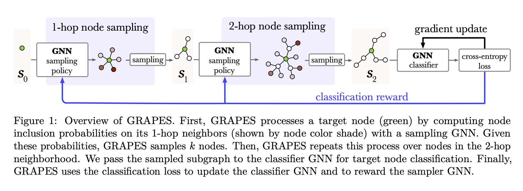
🍇 GRAPES: Learning to Sample Graphs for Scalable Graph Neural Networks 🍇
There's lots of work on sampling subgraphs for GNNs, but relatively little on making this sampling process _adaptive_. That is, learning to select the data from the graph that is relevant for your task.
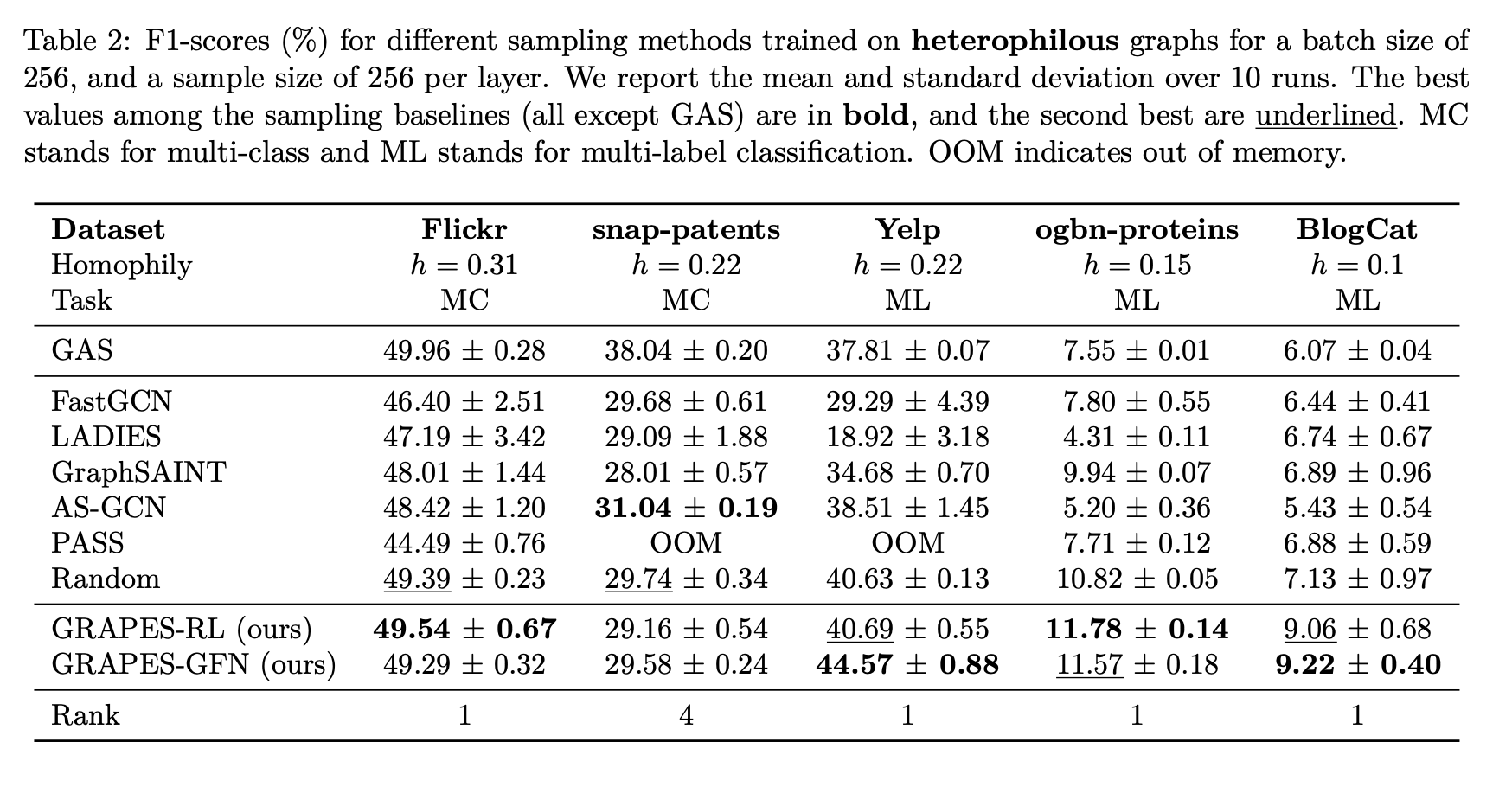
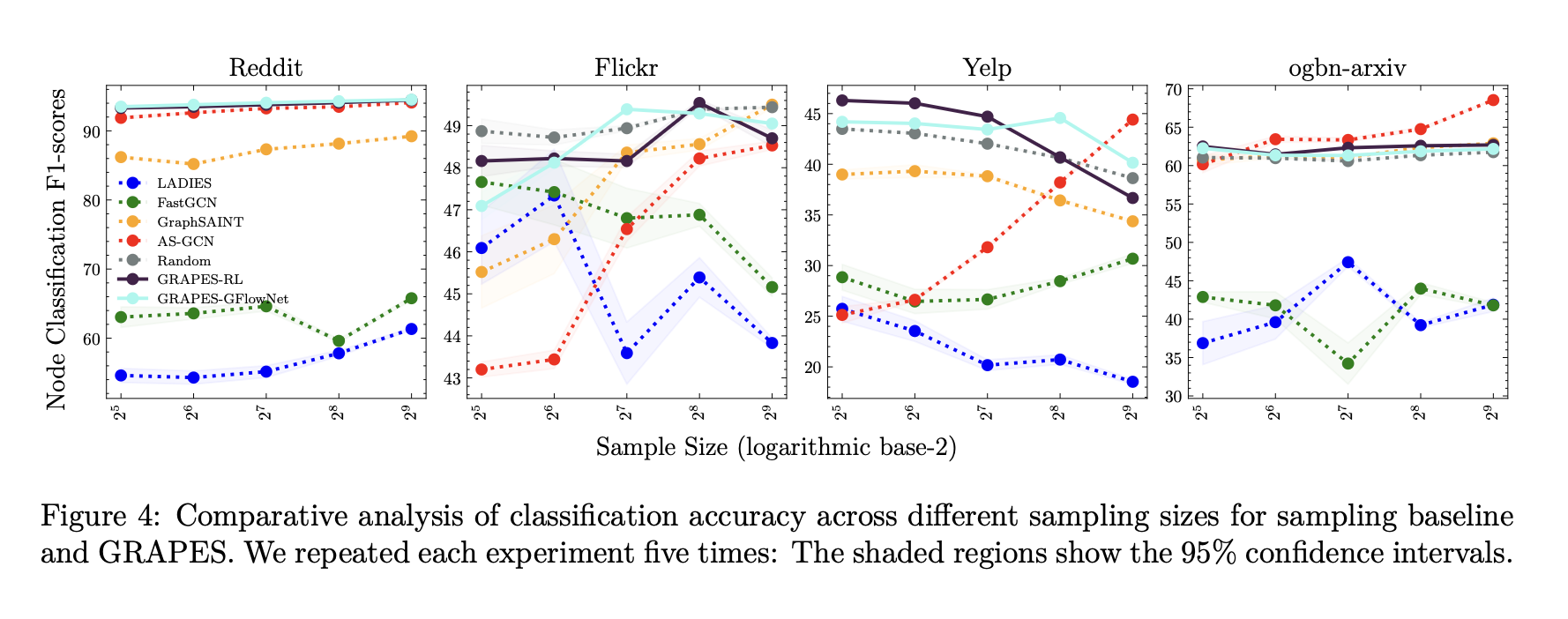
We introduce an RL-based and a GFLowNet-based sampler and show that the approach perf…

A diagram of the GRAPES pipeline. It shows a subgraph being sampled in two steps and being fed to a GNN, with a blue line showing the learning signal. The caption reads Figure 1: Overview of GRAPES. First, GRAPES processes a target node (green) by computing node inclusion probabilities on its 1-hop neighbors (shown by node color shade) with a sampling GNN. Given these probabilities, GRAPES samples k nodes. Then, GRAPES repeats this process over nodes in the 2-hop neighborhood. We pass the sampl…
A results table for node classification on heterophilious graphs. Table 2: F1-scores (%) for different sampling methods trained on heterophilous graphs for a batch size of 256, and a sample size of 256 per layer. We report the mean and standard deviation over 10 runs. The best values among the sampling baselines (all except GAS) are in bold, and the second best are underlined. MC stands for multi-class and ML stands for multi-label classification. OOM indicates out of memory.
Performance of samples vs sampling size showing that GRAPES generally performs well across sample sizes, while other samplers often show more variance across sample sizes. The caption reads Figure 4: Comparative analysis of classification accuracy across different sampling sizes for sampling baseline
and GRAPES. We repeated each experiment five times: The shaded regions show the 95% confidence intervals.
A diagrammatic illustration of a graph classification task used in one of the theorems. The caption reads Figure 9: An example of a graph for Theorem 1 with eight nodes. Red edges belong to E1, features xi and labels yi are shown beside every node. For nodes v1 and v2 we show the edge e12 as an example. As shown, the label of each node is the second feature of its neighbor, where a red edge connects them. The edge homophily ratio is h=12/28 = 0.43.